A paper from June this year showed how to use Cartesian Genetic Programming to play Atari 2600 games. What I find exciting about this is that the system evolves programs. That’s powerful because programs are things we can look at and try to understand as well as run. This post explores the details of the representation used in the paper.
References and links are all at the end of this post.
Evolved programs
The work I’m referring to is by Wilson et al. (2018), called “Evolving simple programs for playing Atari games”. The basic idea is to evolve a game player by:
- having a population of floating point vectors to represent a program (the chromosome, a lot more on this later);
- evaluating the chromosome by playing an Atari game and seeing what score it gets; and
- evolving the population to improve the score.
The paper reports performance at this task which is “competitive with state of the art methods for the Atari benchmark set and require less training time.”
In this post I want to focus on the representation of the program. I’ll get to that in the next section, but first it helps to see the behaviour of a game.
The authors published the source code they used, so I used my laptop to run it (the problem in part is one of throwing chip cycles at it, so my results are going to be limited).
Here’s an example for space invaders:
What you’re looking at here is the behaviour of an evolved program recorded playing a single game of Space Invaders via the Arcade Learning Environment (ALE).
To avoid confusion: this is what I achieved in one run on my laptop, and is not representative of the results reported in the paper. But even so, there’s a hint there of something interesting happening. It only scores 730. For comparison, random behaviour scores 148.
We can look at the program evolved for that game:
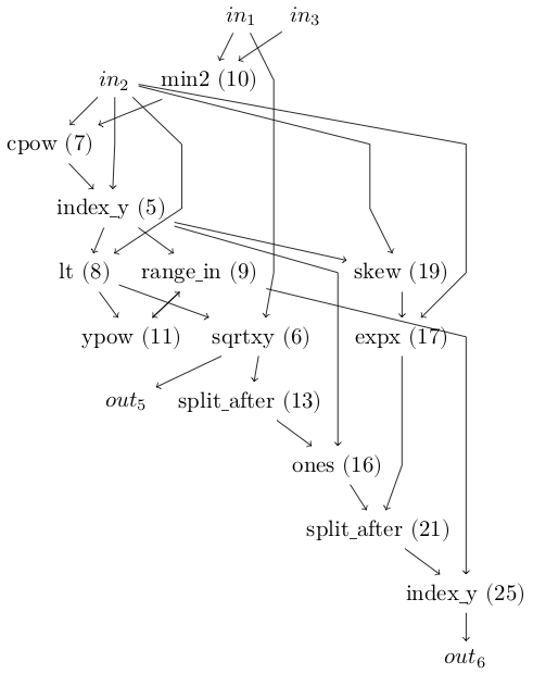
What you’re looking at is a graph of computations. At the top are the inputs, representing the red, green and blue channels of a video frame. At the bottom are the outputs. Space Invaders on the ALE platform has six controls: no-op, fire, left, right, right and fire, and left and fire. In our evolved programme only outputs 5 and 6 are used (left with firing and right with firing).
Between them are compute nodes which are functions. They take as input the output from other functions or the video input. The node inputs and outputs can be matrices or single values.
For example, output 6 receives a value from the index_y function. That, in turn, takes input from split_after and range_in functions. What the functions do doesn’t matter much, but note that they are the fundamental building blocks provided in the experiment. That is, the evolution process isn’t inventing index_y; we’re giving it index_y as one of the functions it can use.
To run the program you compute the output values and the highest one is the winner and that’s the button that gets pushed.
Representing a program
How does that program get represented? Looking at the encoding of that evolved program we see this:
[0.387483, 0.964492, 0.498499, 0.880091, 0.865346, 0.972679, 0.17035, 0.118504, 0.5638, 0.972469, 0.854824, 0.0706383, 0.998166, 0.215527, 0.755458, 0.912714, 0.35665, 0.142379, 0.848166, 0.926213, 0.526343, 0.166038, 0.940983, 0.56913, 0.0884916, 0.401415, 0.169775, 0.350624, 0.0819189, 0.891641, 0.435603, 0.524167, 0.646399, 0.0438218, 0.253205, 0.446265, 0.355821, 0.599058, 0.586079, 0.505821, 0.378716, 0.997763, 0.0286981, 0.105326, 0.502818, 0.390402, 0.398588, 0.778181, 0.78295, 0.361797, 0.420164, 0.291296, 0.963203, 0.00533432, 0.738647, 0.63546, 0.849057, 0.292346, 0.703992, 0.756866, 0.827094, 0.0772889, 0.972571, 0.0944674, 0.271141, 0.970412, 0.27796, 0.640642, 0.300486, 0.231198, 0.0968797, 0.312304, 0.672371, 0.39519, 0.981925, 0.614306, 0.55184, 0.735522, 0.695177, 0.780529, 0.363064, 0.218177, 0.766354, 0.574195, 0.368806, 0.811071, 0.334892, 0.338751, 0.993444, 0.0764086, 0.170724, 0.562696, 0.0194578, 0.323264, 0.801624, 0.908674, 0.469188, 0.628327, 0.126535, 0.456456, 0.0235268, 0.654265, 0.636141, 0.173691, 0.162326, 0.746988, 0.590934, 0.424096, 0.208302, 0.650196, 0.449606, 0.103565, 0.133532, 0.235612, 0.0298292, 0.21659, 0.155102, 0.761937, 0.167632, 0.732491, 0.866052, 0.682638, 0.650841, 0.0782333, 0.230875, 0.688882, 0.155015, 0.37588, 0.0230611, 0.153059, 0.127039, 0.991489, 0.597917, 0.965767, 0.101806, 0.475754, 0.35685, 0.0321371, 0.848377, 0.300844, 0.97208, 0.193615, 0.944256, 0.905844, 0.211629, 0.724031, 0.739358, 0.321951, 0.82216, 0.933464, 0.638504, 0.346732, 0.974737, 0.440503, 0.839242, 0.412772, 0.402766, 0.890078, 0.932978, 0.291289, 0.658856, 0.428769, 0.803972, 0.942145, 0.177263, 0.625429, 0.330744, 0.876799, 0.323458]
That’s a 169 element array, representing the chromosome of a game player.
The “Cartesian” in Cartesian Genetic Programming is because CGP was initially a 2D grid of compute nodes. Each node had a x and y coordinate. However, that appears to have not been necessary, and now CGP uses a 1D array of nodes. That’s why we have a flat array of 169 elements.
But there is structure in the array. It’s like this:
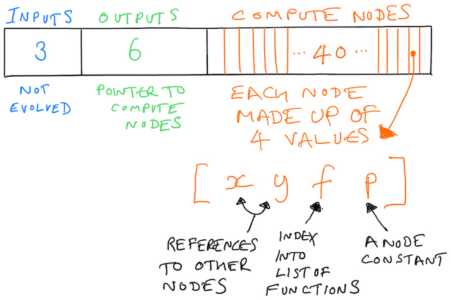
The first three values represent the inputs. The system does not evolve the inputs, and from our perspective they exist as targets for other nodes to point at. Remember that we’re building up a graph, and nodes in the graph need to reference other nodes.
The next batch of values represent the outputs. A value here is a pointer towards a compute note. To draw the graph you take an output node, see what it points to, and then walk the graph. These values are evolved, meaning what an output points to can change throughout evolution.
That’s 9 of the 169 values covered. What follows next is 40 (in this example) compute nodes each made up of 4 values. That’s 160 values, getting us to the 169 total.
Those four values control which function the node represents and what inputs it takes. Every function also receives a third value as input, which is p in the diagram above. Many functions ignore the value, but it is used sometimes, such as a range function.
Each one of those four values is a node (or “gene”). We evolve these values.
Walking the graph
I found it helpful to trace an output to see how the graph builds up. So let’s take a look at how we get to index_y connected to out6.
Output 6 will be the 9th value in our array: we skip the three inputs then count six forward. It has the value 0.5638, which we can see in code (using the Julia language):
# `b` is the array of 169 values
julia> b[9]
0.5638
This number is a reference to a compute node. We scale the value to the number of nodes we have (43, including the inputs):
julia> node_index = Int64(ceil(b[9] * 43))
25
So we know we need to see what compute node 25 is all about.
In fact, you know what node 25 is all about because I’ve labelled the node number on the program graph. Still, let’s work the numbers to see how this pans out.
To make this easier to read we can reshape the chromosome input into groups of 4, adding in placeholders for the input nodes:
julia> nin = 3
3

julia> nout = 6
6

julia> num_nodes = 40
40

julia> compute_nodes = reshape(b[(nin+nout+1):end], (4, num_nodes))'
40×4 Array{Float64,2}:
 0.972469    0.854824   0.0706383  0.998166
 0.215527    0.755458   0.912714   0.35665
 0.142379    0.848166   0.926213   0.526343
...

julia> input_nodes = zeros(3, 4)
3×4 Array{Float64,2}:
 0.0  0.0  0.0  0.0
 0.0  0.0  0.0  0.0
 0.0  0.0  0.0  0.0

julia> nodes = [input_nodes; compute_nodes]
43×4 Array{Float64,2}:
 0.0         0.0        0.0        0.0
 0.0         0.0        0.0        0.0
 0.0         0.0        0.0        0.0
 0.972469    0.854824   0.0706383  0.998166
 0.215527    0.755458   0.912714   0.35665
...
The four values for node 25 are:
julia> nodes[25,:]
4-element Array{Float64,1}:
 0.323264
 0.801624
 0.908674
 0.469188
The 3rd one of those numbers is the function (the 1st and 2nd are pointers to other nodes to use as input; the 4th is the extra constant input parameter). The system has a list of 54 functions, and we scale 0.908674 into that list and find the function is f_index_y:
julia> f_index = Int64(ceil(nodes[25, 3] * 54))
50

julia> CGP.Config.functions[50]
f_index_y (generic function with 8 methods)
Next we need to find out which other nodes are input to node 25. That’s similar to how we found the node in first place, but there’s a complication. In CGP there’s a parameter called r (I read r as “range”) which controls how far forward a node can look for connections. For example, if we had 15 nodes and wanted a 10% range, the 5th node could accept connections from anything before it, and 10% of the remaining 10 nodes:
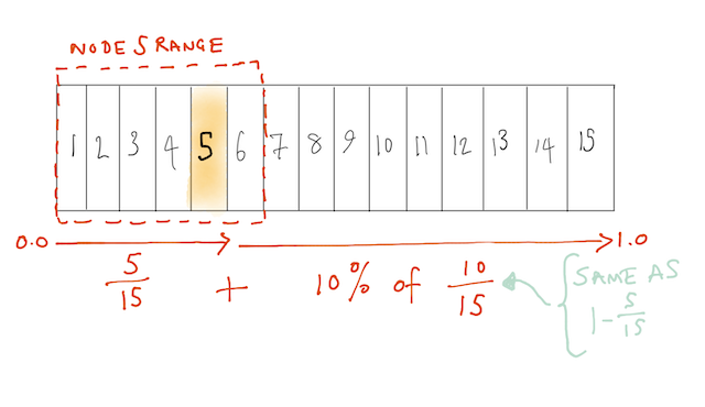
I don’t yet know what the motivation is for this range limiting. In this work the range was 10% (0.1) and we can compute it for the connections to node 25:
julia> frac = 25 / 43
0.5813953488372093

julia> range = frac + 0.1 * (1 - frac)
0.6232558139534884

# The 1st and 2nd elements tell us which nodes are inputs:
julia> nodes[25, 1:2] * range * 43
2-element Array{Float64,1}:
  8.66348
 21.4835

 # ...rounded:
 julia> map(p -> Int64(round(p * range * 43)), nodes[25, 1:2])
2-element Array{Int64,1}:
  9
 21
So node 25 receives inputs from nodes 9 and 21. OK, that’s probably too much detail for most people, but I like to know how the numbers work out. We could now recurse and look at the inputs and functions for nodes 9 and 21, but I think you get the idea.
Neat tricks
There’s more to it than that, and I don’t fully understand everything in the CGP software yet. But one thing I was wondering was: where’s outputs 1, 2, 3 and 4 on the diagram?
I can imagine trimming out long graphs of nodes. Or nodes that lead to no inputs. But there’s another trick. The figure I showed above, with just output 5 and 6 on it, is only showing outputs used during a game. That is: count how many times an output is triggered, and if it’s never triggered, don’t draw the node.
Evolution
With all of that in hand, we can see how a population of floating point numbers can represent programs. Evaluating those programs by playing a game allows us to score them. We can then produce new offspring by mutating the best players. And round we go until we’ve had enough.
Context: why is this interesting?
In 2015 Nature published a paper from DeepMind which showed deep-reinforcement learning used to play Atari games. That is, they used deep neural networks fed with video frames and the game score as it played. It was a big deal: it achieved a level comparable with professional human gamers and didn’t require tweaking for each game. It set the stage for the tacking the game of Go.
That’s one algorithm (a “deep Q-network”), but as we’ve seen, other algorithms are available. The above work shows a CGP alternative, with competitive performance. But notice that the solution evolved is something we can inspect.
I find all of this interesting for various reasons:
- the rich representation you can use as building blocks;
- applying evolutionary computing techniques to the problem; and
- the generation of simple programs which might be things we can understand.
References
Papers
Wilson et al (2018) Evolving simple programs for playing Atari games arXiv:1806.05695v1 (PDF)
Mnih et al (2015) Human-level control through Deep Reinforcement Learning doi:10.1038/nature14236 (PDF)
Silver et al. (2016) Mastering the game of Go with deep neural networks and tree search doi:10.1038/nature16961
Code
CGP.jl, the software referenced in the CGP Atari paper.
My fork of CGP.jl to work around a probably minor problem with the above software at the time. The problem is fixed in the
julia1branch of the original code, so probably ignore my fork.ALE, the Arcade Learning Environment.
Additional notes
Evolutionary algorithm outperforms deep-learning machines at video games, Technology Review.
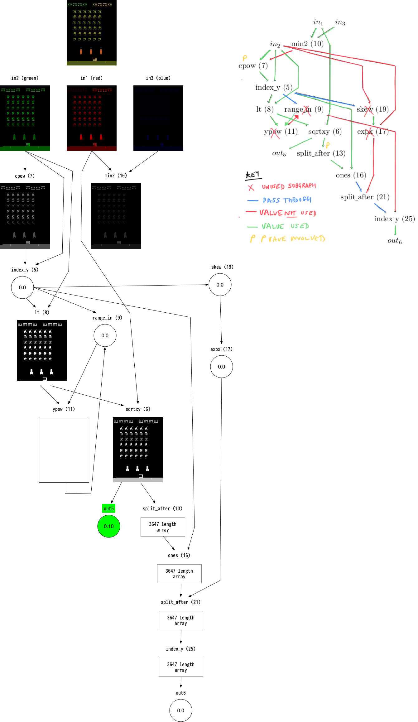
Visualization of one frame of the game for the program graph shown in this post. I may well have made some errors in that diagram as I produced it by hand (definitely something to automate as I don’t fancy doing that again). To make sense of the functions you need to read functions.jl, especially
load_functions; atari.yml for the function definitions; and chromosome.jl for how the outputs are processed from nodes.